Machine Learning Tutorial #1: Preprocessing
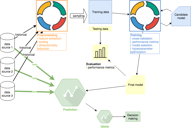
In this machine learning tutorial, I will explore 4 steps that define a typical machine learning project: Preprocessing, Learning, Evaluation, and Prediction (deployment). In this first part, I will complete the Preprocessing step. Other tutorials in this series: #1 Preprocessing (this article), #2 Training, #3 Evaluation , #4 Prediction
I will use stock price data as the main dataset. There are a few reasons why this is a good choice for the tutorial:
- The dataset is public by definition and can be easily downloaded from multiple sources so anyone can replicate the work.
- Not all features are immediately available from the source and need to be extracted using domain knowledge, resembling real life.
- The outcome of the project is highly uncertain which again simulates real life. Billions of dollars are thrown at the stock price prediction problem every year and the vast majority of projects fail. This tutorial is therefore not about creating a magical money-printing machine; it is about replicating the experience a machine learning engineer might have with a project.
All code is located at the following Github repo. The file “preprocessing.py” drives the analysis. Python 3.6 is recommended and the file includes directions to setup all necessary dependencies.
First we need to download the dataset. I will somewhat arbitrarily choose the Microsoft stock data (source: Yahoo Finance). I will use the entire available history which at the time of writing includes 3/13/1986 — 7/30/2018. The share price performed as follows during this period:
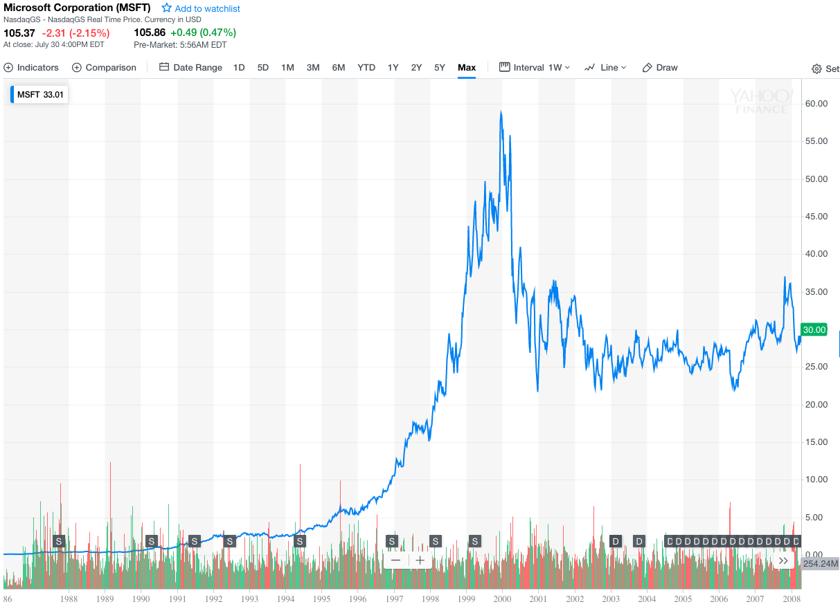
The price movement is interesting because it exhibits at least two modes of behavior:
- the steep rise until the year 2000 when tech stocks crashed
- the sideways movement since 2000
This makes for a number of interesting machine learning complexities such as the sampling of training and testing data.
Data Cleaning
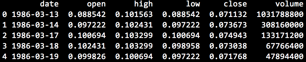
After some simple manipulations and loading of the csv data into pandas DataFrame, we have the following dataset where open, high, low and close represent prices on each date and volume the total number of shares traded.
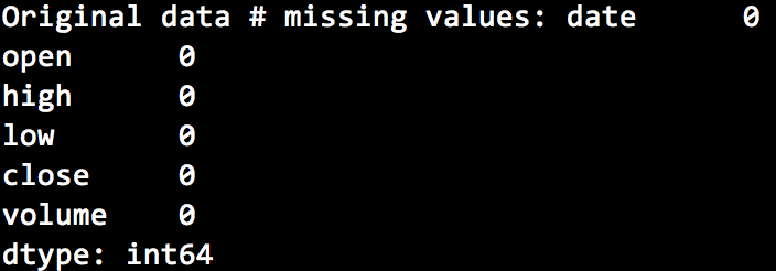
Missing values are not present which I confirmed by running the following command:
missing_values_count = df.isnull().sum()
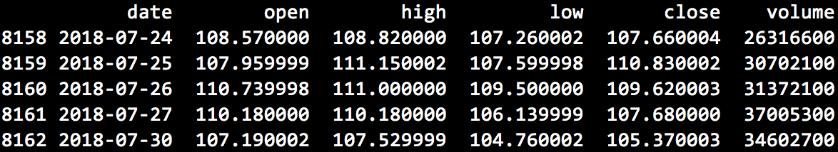
Outliers are the next topic I need to address. The key point to understand here is that our dataset now includes prices but prices are not the metric I will attempt to forecast because they are measured in absolute terms and therefore harder to compare across time and other assets. In the tables above, the first price available is ~$0.07 while the last is $105.37.
Instead, I will attempt to forecast daily returns. For example, at the end of the second trading day the return was +3.6% (0.073673/0.071132). I will therefore create a return column and use it to analyze possible outliers.
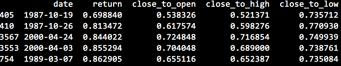
The 5 smallest daily returns present in the dataset are the following:
And 5 largest daily returns:
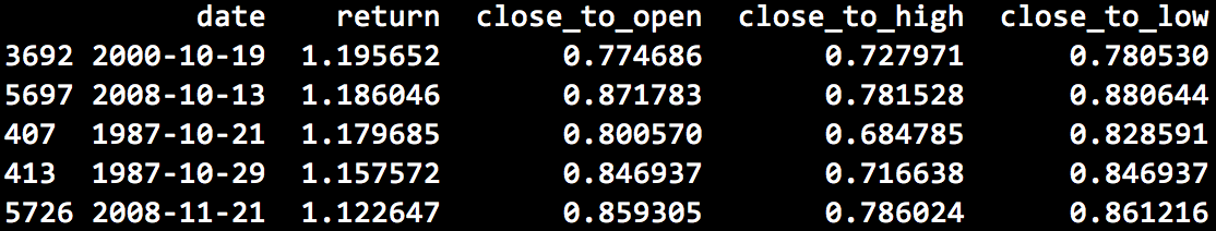
The most negative return is -30% (index 405) and the largest is 20% (index 3692). Normally, a further domain-specific analysis of the outliers is necessary here. I will skip it for now and assume this tutorial outlines the process for illustrative purposes only. Generally, the data appears to make sense given that in 1987 and 2000 market crashes took place associated with extremely volatility.
The same analysis would be required for open, high, low and volume columns. Admittedly, data cleaning was somewhat academic because Yahoo Finance is a very widely used and reliable source. It is still a useful exercise to understand the data.
Target Variable Selection
We need to define what our ML algorithms will attempt to forecast. Specifically, we will forecast next day’s return. The timing of returns is important here so we are not mistakenly forecasting today’s or yesterday’s return. The formula to define tomorrow’s return as our target variable is as follows:
df["y"] = df["return"].shift(-1)
Feature Extraction
Now I will turn to some simple transformations of the prices, returns and volume to extract features ML algorithms can consume. Finance practitioners have developed 100s of such features but I will only show a few. Hedge funds spent the vast majority of time on this step because ML algorithms are generally only as useful as the data available, aka. “garbage in, garbage out”.
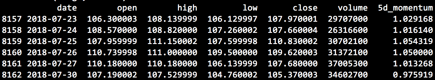
One feature we might consider is how today’s closing price relates to that of 5 trading days ago (one calendar week). I call this feature “5d_momentum”:
df[“5d_momentum”] = df[“close”] / df[“close”].shift(5)
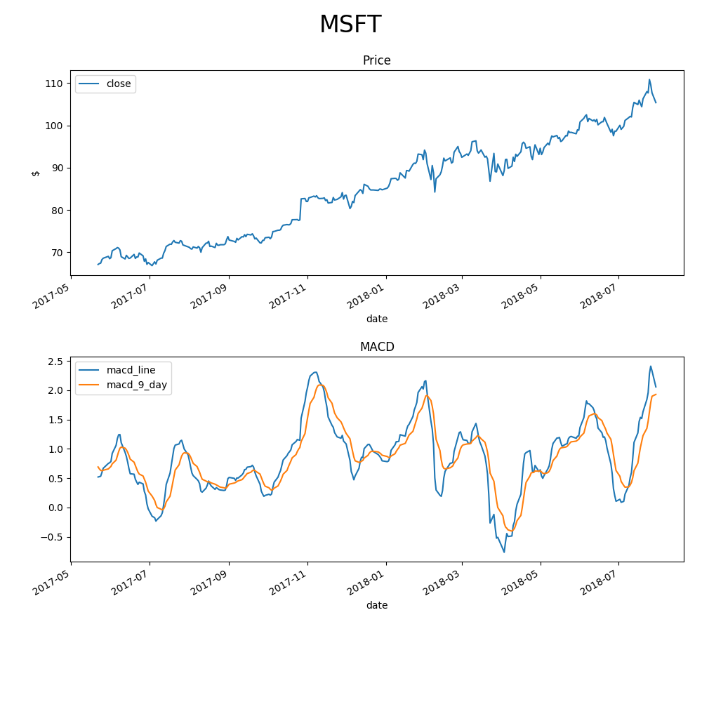
One typical trend following feature is MACD (Moving Average Convergence/Divergence Oscillator). The strengths of pandas shine here because MACD can be created in only 4 lines of code. The chart of the MACD indicator is below. On the lower graph, a typical buy signal would be the blue “macd_line” crossing above the orange line representing a 9-day exponential moving average of the “macd_line”. The inverse would represent a sell signal.
The python code “generate_features.py” located in the Github repo mentioned above includes additional features we might consider. For example:
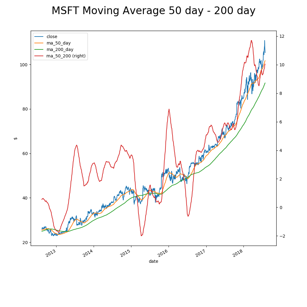
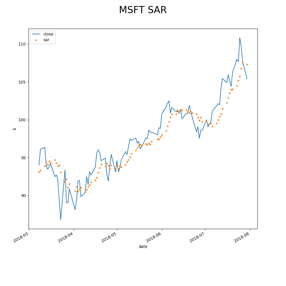
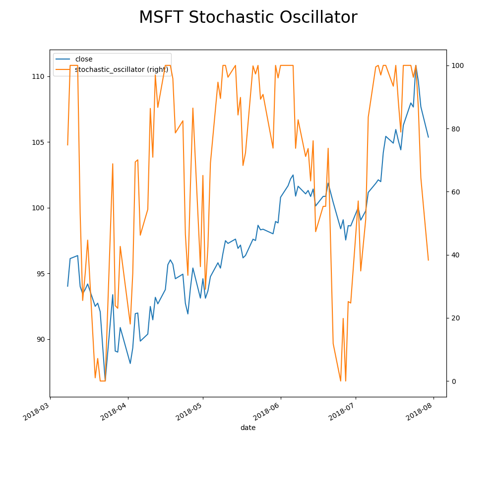
At the end of the feature extraction process, we have the following features:
['return', 'close_to_open', 'close_to_high', 'close_to_low', 'macd_diff', 'ma_50_200', 'sar', 'stochastic_oscillator', 'cci', 'rsi', '5d_volatility', '21d_volatility', '60d_volatility', 'bollinger', 'atr', 'on_balance_volume', 'chaikin_oscillator']
Sampling
We need to split the data into training and testing buckets. I cannot stress enough that the testing dataset should never be used in the Learning step. It will be used only in the Evaluation step so that performance metrics are completely independent of training and represent an unbiased estimate of actual performance.
Normally, we could randomize the sampling of testing data but time series data is often not well suited for randomized sampling. The reason being that would would bias the learning process. For example, randomization could produce a situation where the data point from 1/1/2005 is used in the Learning step to later forecast a return from 1/1/2003.
I will therefore choose a much simpler way to sample the data and use the first 7000 samples as training dataset for Learning and the remaining 962 as testing dataset for Evaluation.
Both datasets will be saved as csv files so we conclude this part of the ML tutorial by storing 4 files (MSFT_X_learn.csv, MSFT_y_learn.csv, MSFT_X_test.csv, MSFT_y_test.csv). These will be consumed by the next steps of this tutorial.
Scaling
Feature scaling is used to reduce the time to Learn. This typically applies to stochastic gradient descent and SMV.
The open source sklearn package will be used for most additional ML application so I will start using it here to scale all features to have zero mean and unit variance:
from sklearn import preprocessing
scaler_model = preprocessing.StandardScaler().fit(X_train)
X_train_scaled = scaler_model.transform(X_train)
X_test_scaled = scaler_model.transform(X_test)
It is important that data sampling takes place before features are modified to avoid any training to testing data leakage.
Dimensionality Reduction
At this stage, our dataset 17 features. The number of features has a significant impact on the speed of learning. We could use a number of techniques to try to reduce the number of features so that only the most “useful” features remain.
Many hedge funds would be working with 100s of features at this stage so dimensional reduction would be critical. In our case, we only have 17 illustrative features so I will keep them all in the dataset until I explore the learning times of different algorithms.
Out of curiosity however, I will perform Principal Component Analysis (PCA) to get an idea of how many features we could create from our dataset without losing meaningful explanatory power.
from sklearn.decomposition import PCA
sk_model = PCA(n_components=10)
sk_model.fit_transform(features_ndarray)
print(sk_model.explained_variance_ratio_.cumsum())
 [0.30661571 0.48477408 0.61031358 0.71853895 0.78043556 0.83205298
 0.8764804  0.91533986 0.94022672 0.96216244]
The first 8 features explain 91.5% of data variance. The downside of PCA is that new features are located in a lower dimensional space so they no longer correspond the real-life concepts. For example, the first original feature could be “macd_line” I derived above. After PCA, the first feature explains 31% of variance but we not longer have any logical description for what the feature represents in real life.
For now, I will keep all features 17 original features but note that if the learning time of algorithms is too slow, PCA will be helpful.
Other tutorials in this series: #1 Preprocessing (this article), #2 Training, #3 Evaluation , #4 Prediction