Machine Learning Tutorial #2: Training
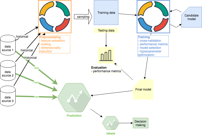
This second part of the ML Tutorial follows up on the first Preprocessing part. All code is available in this Github repo. Other tutorials in this series: #1 Preprocessing, #2 Training (this article), #3 Evaluation , #4 Prediction
I concluded Tutorial #1 with 4 datasets: training features, testing features, training target variables, and testing target variables. Only training features and and training target variables will be used in this Tutorial #2. The testing data will be used for evaluation purposes in Tutorial #3.
Performance Metrics
We are focused on regression algorithms so I will consider 3 most often used performance metrics
- Mean Absolute Error (MAE)
- Mean Squared Error (MSE)
In practice, a domain-specific decision could be made to supplement the standard metrics above. For example, investors are typically more concerned about significant downside errors rather than upside errors. As a result, a metric could be derived that overemphasizes downside errors corresponding to financial losses.
Cross Validation
I will return to the same topic I addressed in Preprocessing. Due to the nature of time series data, standard randomized K-fold validation produces forward looking bias and should not be used. To illustrate the issue here, let’s assume that we split 8 years of data into 8 folds, each representing one year. The first training cycle will use folds #1–7 for training and fold #8 for testing. The next training cycle may use folds #2–8 for training and fold #1 for testing. This is of course unacceptable because we are using data from years 2–7 to forecast year 1.
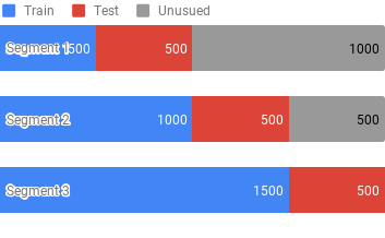
Our cross validation must respect the temporal sequence of the data. We can use Walk Forward Validation or simply multiple Train-Test Splits. For illustration, I will use 3 Train-Test splits. For example, let’s assume we have 2000 samples sorted by timestamp from the earliest. Our 3 segments would look as follows:
Model Selection
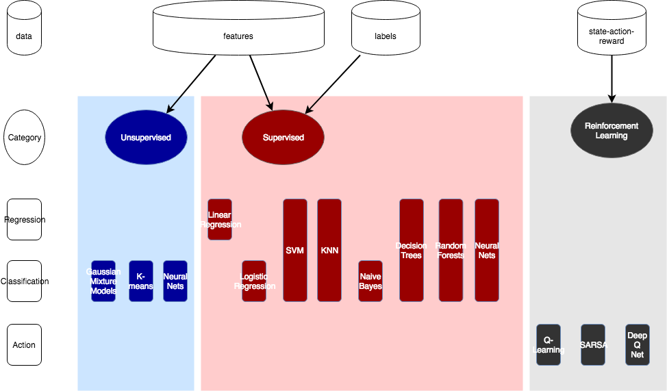
In this section, I will select the models to train. The “Supervised” algorithms section (red section in the image above) is relevant because the dataset contains both features and labels (target variables). I like to follow Occam’s razor when it comes to algorithms selection. In other words, start with the algorithm that exhibits the fastest times to train and the greatest interpretability. Then we can increase complexity.
I will explore the following algorithms in this section:
- Linear Regression: fast to learn, easy to interpret
- Decision Trees: fast to learn (requires pruning), easy to interpret
- Neural Networks: slow to learn, hard to interpret
Linear Regression
Starting with linear regression is useful to see if we can “get away” with simple statistics to achieve our goal before diving into complex machine learning algorithms. House price forecasting with clearly defined features is an example where linear regression often works well and using more complex algorithms is unnecessary.
Training a linear regression model using sklearn is simple:
from sklearn import linear_model
model = linear_model.LinearRegression()
model.fit(X_train, y_train)
y_pred = model.predict(X_test)
Initial results yielded nothing remotely promising so I took another step and transformed features further. I created polynomial and nonlinear features to account for nonlinear relationships. For example, features [a, b] become [1, a, b, a², ab, b²] in the case of degree-2 polynomial.
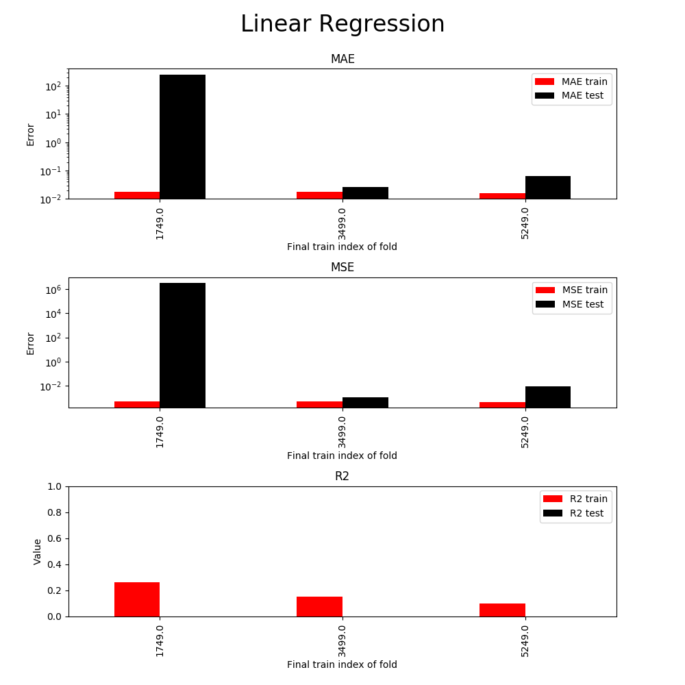
The x-axis represents 3 cross validation segments (the fold 1st uses 1749 samples for training and 1749 for testing, the 2nd uses 3499 for training and 1749 for testing, and the last uses 5249 for training and 1749 for testing). Clearly, the results suggest that the linear model is not useful in practice. At this stage I have at least the following options:
- Ridge regression: addresses overfitting (if any)
- Lasso linear: reduces model complexity
At this point, I don’t believe that any of the options above will meaningfully impact the outcome. I will move on to other algorithms to see how they compare.
Before moving on, however, I need to set expectations. There is a saying in finance that successful forecasters only need to be correct 51% of the time. Financial leverage can be used to magnify results so being just a little correct produces impactful outcomes. This sets expectations because we will never find algorithms that are constantly 60% correct or better in this domain. As a result, we expect low R² values. This needs to be said because many sample projects in machine learning are designed to look good, which we can never match in real-life price forecasting.
Decision Tree
Training a decision tree regressor model using sklearn is equally simple:
from sklearn import tree
model = tree.DecisionTreeRegressor()
model.fit(X_train, y_train)
y_pred = model.predict(X_test)
The default results for the fit function above almost always overfit. Decision trees have a very expressive hypothesis space so they can represent almost any function when not pruned. R² for training data can easily become perfect 1.0 while for testing data the result will be 0. We therefore need to use the max_depth argument of scikit-learn DecisionTreeRegressor to enforce that the tree generalizes well for test data.
One of the biggest advantages of decision trees is their interpretability: see many useful visualization articles using standard illustrative datasets.
Neural Networks
Scikit-learn makes simple neural network training just as simple as building a decision tree:
from sklearn.neural_network import MLPRegressor
model = MLPRegressor(hidden_layer_sizes=(200, 200), solver="lbfgs", activation="relu")
model.fit(X_train, y_train)
y_pred = model.predict(X_test)
Training a neural net with 2 hidden layers (of 200 units each) and polynomial features starts taking tens of seconds on an average laptop. To speed up the training process in the next section, I will step away from scikit-learn and use Keras with TensorFlow backend.
Keras API is equally simple. The project even includes wrappers for scikit-learn to take advantage of scikit’s research libraries.
from keras.models import Sequential
from keras.layers import Dense
model = Sequential()
input_size = len(X[0])
model.add(Dense(200, activation="relu", input_dim=input_size))
model.add(Dense(200, activation="relu"))
model.add(Dense(1, activation="linear"))
model.compile(optimizer="adam", loss="mse")
model.fit(X_train, y_train, epochs=25, verbose=1)
y_pred = model.predict(X_test)
Hyperparameter Optimization
The trick to doing hyperparameter optimization is to understand that parameters should not be treated independently. Many parameters interact with each other which is why exhaustive grid search is often performed. However, grid search is that it becomes expensive very quickly.
Decision Tree
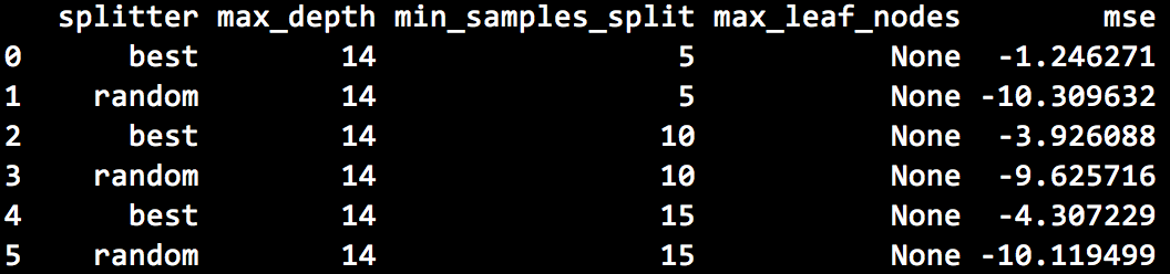
Our decision tree grid search will iterate over the following inputs:
- splitter: strategy used to split nodes (best or random)
- max depth of the tree
- min samples per split: the minimum number of samples required to split an internal node
- max leaf nodes: number or None (allow unlimited number of leaf nodes)
Illustrative grid search results are below:
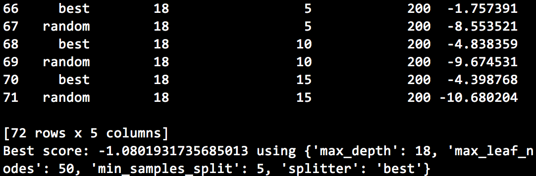
Performance using the best parameters:
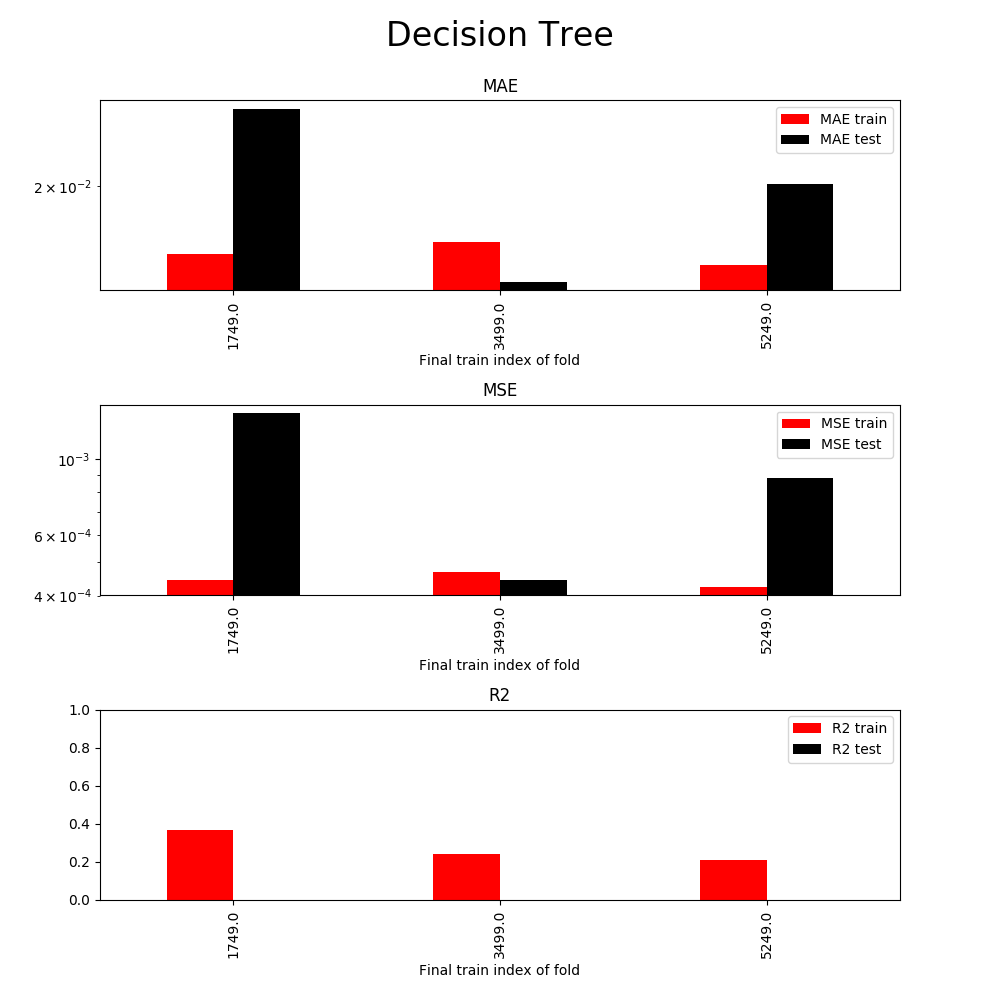
Again, the results do not seem to be very promising. They appear to be better than linear regression (lower MAE and MSE) but R² is still too low to be useful. I would conclude, however, that the greater expressiveness of decision trees is useful and I would discard the linear regression model at this stage.
Neural Networks
Exploring the hyperparameters of the neural net build by Keras, we can alter at least the following parameters:
- number of hidden layers and/or units in each layer
- model optimizer (SGD, Adam, etc)
- activation function in each layer (relu, tanh)
- batch size: the number of samples per gradient update
- epochs to train: the number of iterations over the entire training dataset
Illustrative grid search results are below:
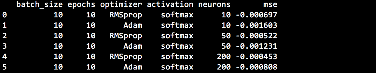
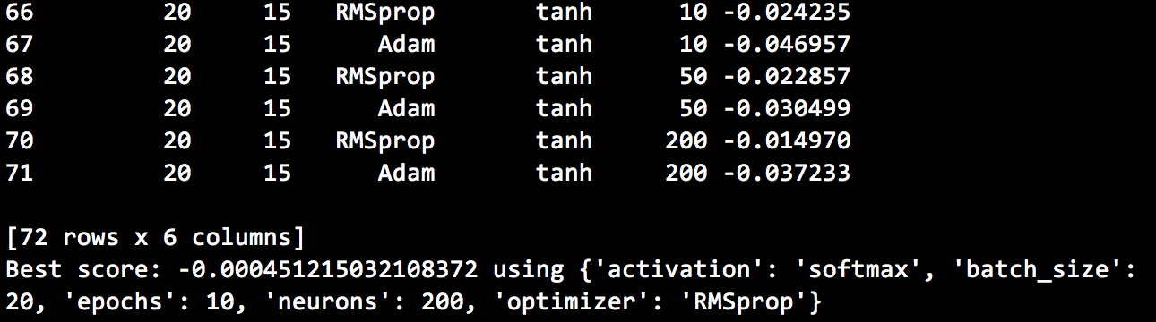
Using the best parameters, we obtain the following performance metrics:
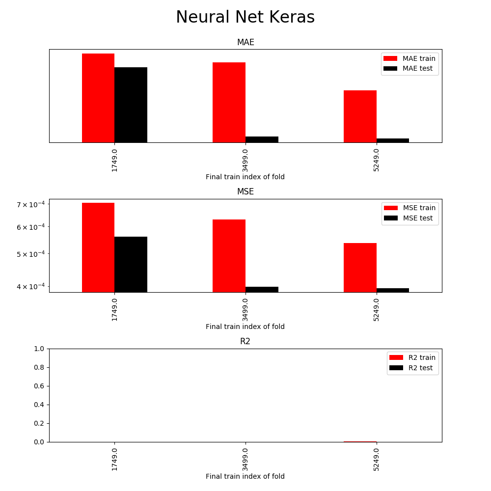
Neural net and decision tree results are similar which is common. Both algorithms have very expressive hypothesis spaces and often produce comparable results. If I achieve comparable results, I tend to use the decision tree model for its faster training times and greater interpretability.
Project Reflection
At this stage it becomes clear that no model can be used in production. While the decision tree model appears to perform the best, its performance on testing data is still unreliable. At this stage, it would be time to go back and find additional features and/or data sources.
As I mentioned in the first Preprocessing Tutorial, finance practitioners might spend months sourcing data and building features. Domain-specific knowledge is crucial and I would argue that financial markets exhibit at least the Weak-Form of Efficient Market Hypothesis. This implies that future stock returns cannot be predicted from past price movements. I have used only past price movements to develop the models above so practitioners would notice already in the first tutorial that results would not be promising.
For the sake of completing this tutorial, I will go ahead and save the decision tree model and use it for illustrative purposes in the next sections of this tutorial (as if it were the Final production model):
pickle.dump(model, open("dtree_model.pkl", "wb"))
Important: there are known security vulnerabilities in the Python pickle library. To stay on the safe side, the key takeaway is to never unpickle data you did not create.
Tools
Tooling is a common question but often not critical until the project is composed of tens of thousands of examples and at least hundreds of features. I typically start with scikit-learn and move elsewhere when performance becomes the bottleneck. TensorFlow, for example, is not just a deep learning framework but also contains other algorithms such as LinearRegressor. We could train Linear Regression above with TensorFlow and GPUs if scikit-learn does not perform well enough.
Other tutorials in this series: #1 Preprocessing, #2 Training (this article), #3 Evaluation , #4 Prediction