Machine Learning Tutorial #3: Evaluation
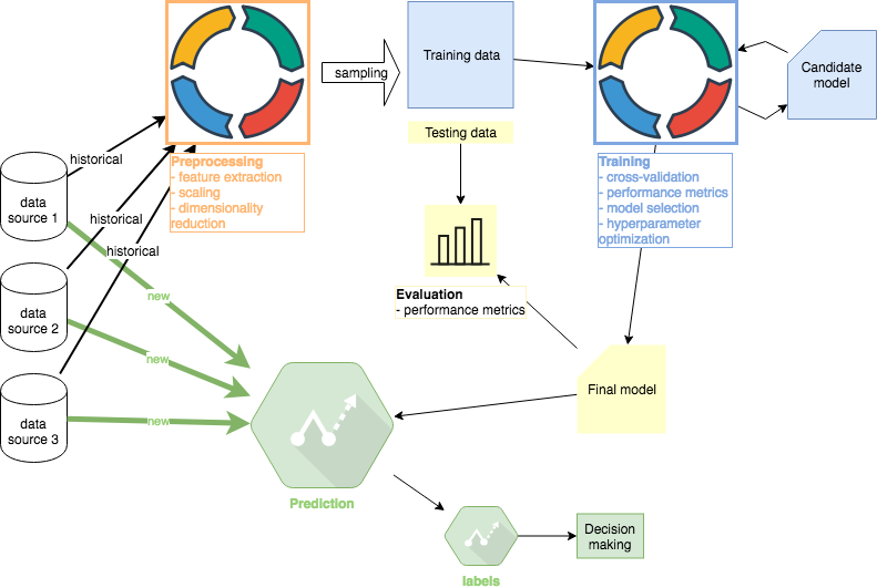
In this third phase of the series, I will explore the Evaluation part of the ML project. I will reuse some of the code and solutions from the second Training phase. However, it is important to note that the Evaluation phase should be completely separate from training except for using the final model produced in the Training step. Other tutorials in this series: #1 Preprocessing, #2 Training, #3 Evaluation (this article), #4 Prediction. Github code.
Performace Metrics
The goal of this section is to determine how our model from the Training step performs on real life data it has not learned from. First, we have to load the model we saved as the Final model:
model = pickle.load(open("dtree_model.pkl", "rb"))
>>> model
DecisionTreeRegressor(criterion='mse', max_depth=3, max_features=None, max_leaf_nodes=None, min_impurity_decrease=0.0, min_impurity_split=None, min_samples_leaf=1, min_samples_split=5, min_weight_fraction_leaf=0.0, presort=False, random_state=1, splitter='best')
Next, we will load the testing data we created in the Preprocessing part of this tutorial. The primary reason why I keep the Evaluation section separate from Training is precisely this step. I keep the code separate as well to ensure that no information from training leaks into evaluation. To restate, we should have not seen the data used in this section at any point until now.
X = pd.read_csv("X_test.csv", header=0)
y = pd.read_csv("y_test.csv", header=0)
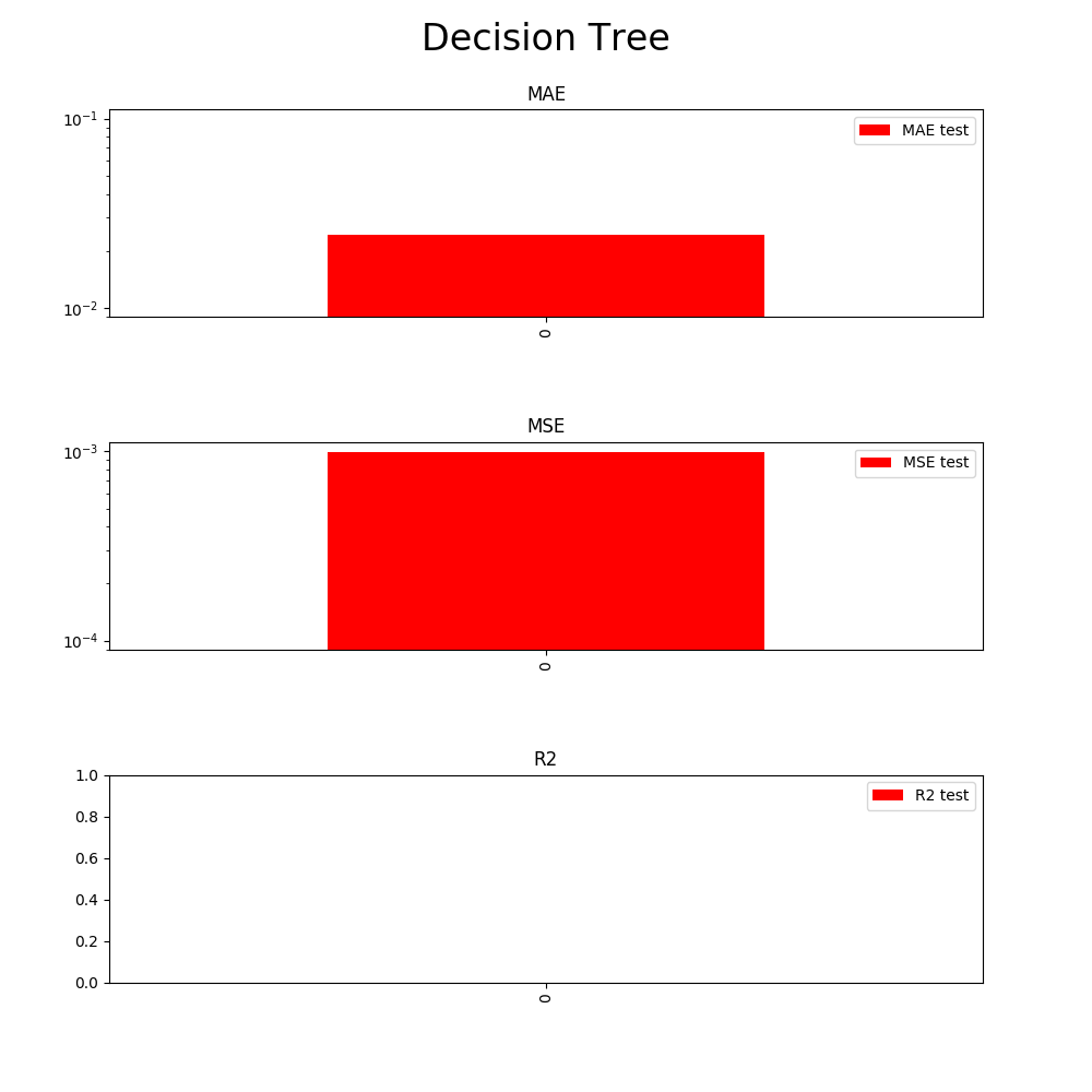
At this stage, we may perform additional performance evaluation on top of the Training step. However, I will stick to the metrics used previously: MAE, MSE, R2.
Commentary
We have known that our model does not perform well enough in practice from the previous tutorial already. However, as I mentioned before, I went ahead and used it for illustrative purposes here in order to complete the tutorial and to explain the kind of thinking involved in real life projects where performance is not always ideal out of the box as many toy datasets would make one think.
The key comparison is how well does our model evaluate relative to the training phase. In the case of models ready for production, I would expect the performance in the Evaluation step to be comparable to those of testing folds in the Training phase.
Comparing the last training test fold here (5249 datapoints used to train) and the Evaluation results above:
- MAE: final Training phase ~10^-2. Evaluation phase ~10^-2
- MSE: final Training phase ~10^-4. Evaluation phase ~10^-3
- R²: final Training phase ~0. Evaluation phase ~0
The performance on dataset the model has never seen before is reasonably similar. Nonetheless, overfitting is still something to potentially address. If we had a model ready for production from the Training phase, we would be reasonably confident at this stage that it would perform as we expect on out of sample data.
Other tutorials in this series: #1 Preprocessing, #2 Training, #3 Evaluation (this article), #4 Prediction