Google Colab and Auto-sklearn with Profiling

Published: 2021-03-20

This article is a follow up to my previous tutorial on how to setup Google Colab and auto-sklean. Here, I will go into more detail that shows auto-sklearn performance on an artificially created dataset. The full notebook gist can be found here.

First, I generated a regression dataset using scikit learn.

X, y, coeff = make_regression(
    n_samples=1000,
    n_features=100,
    n_informative=5,
    noise=0,
    shuffle=False,
    coef=True
)

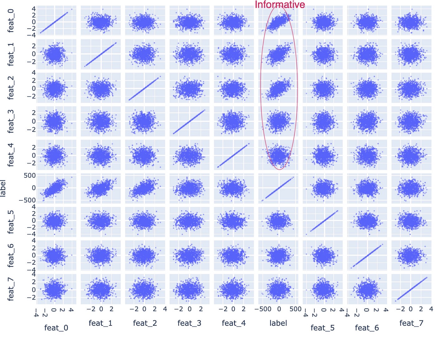
This generates a dataset with 100 numerical features where the first 5 features are informative (these are labeled as “feat_0” to “feat_4”). The rest (“feat_5” to “feat_99”) are random noise. We can see this in the scatter matrix above where only the first 5 features show a correlation with the label.

We know that this is a simple regression problem which could be solved using a linear regression perfectly. However, knowing what to expect helps us to verify the performance of auto-sklearn which trains its ensemble model using the following steps:

import autosklearn.regressionautoml = autosklearn.regression.AutoSklearnRegressor(
    time_left_for_this_task=300,
    n_jobs=-1
)
automl.fit(
    X_train_transformed,
    df_train["label"]
)

I also created random categorical features which are then one-hot-encoded into a feature set “X_train_transformed“. Running the AutoSklearnRegressor for 5 minutes (time_left_for_this_task=300) produced the following expected results:

predictions = automl.predict(X_train_transformed)
r2_score(df_train["label"], predictions)
>> 0.999
predictions = automl.predict(X_test_transformed)
r2_score(df_test["label"], predictions)
>> 0.999

A separate pip package PipelineProfiler helps us visualize the steps auto-sklearn took to achieve the result:

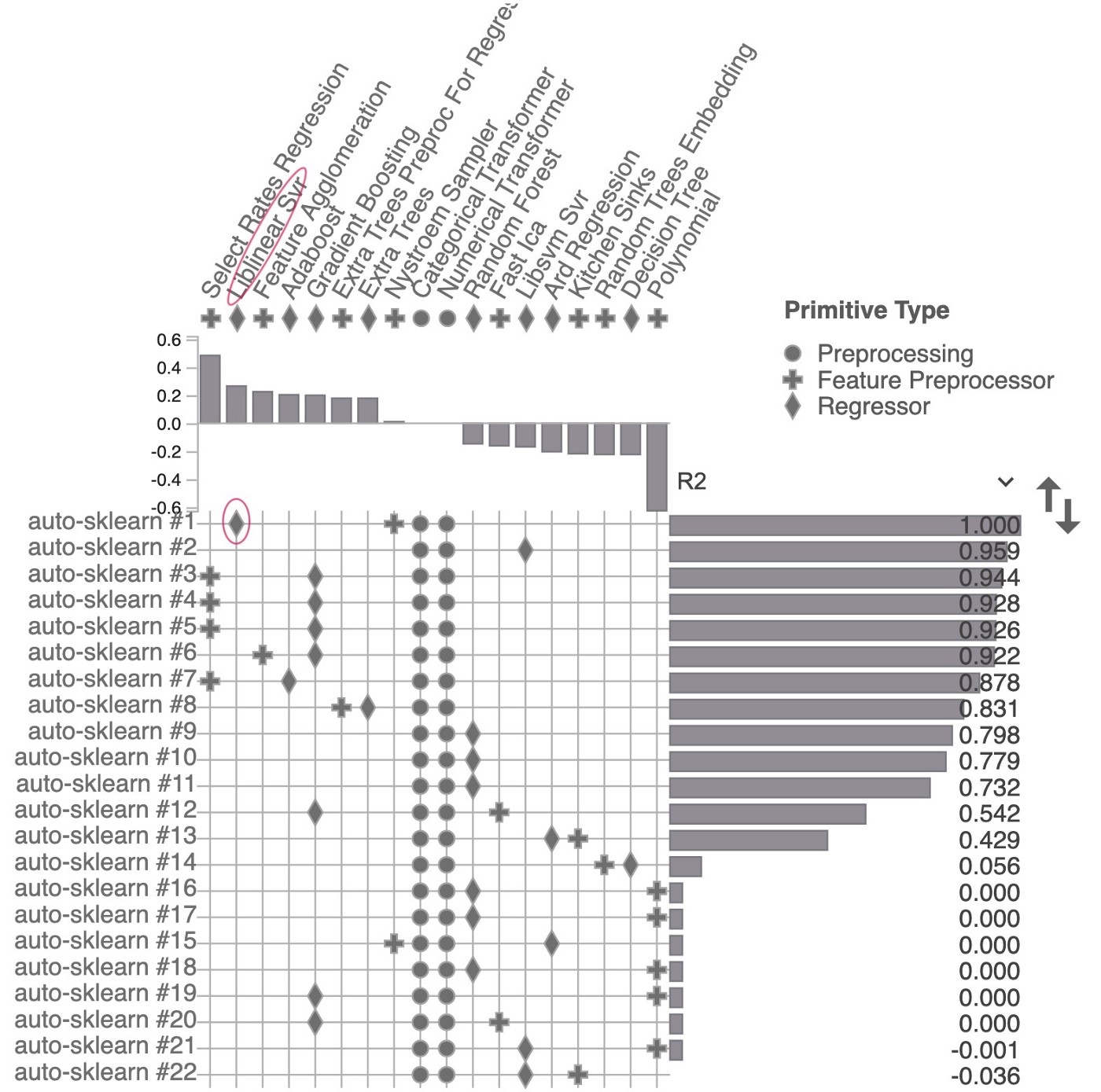
Above we can see the attempts auto-sklearn made to generate the best emsemble of models within the 5 minute constraint I set. The best model found was Liblinear SVM, which produced R2 of nearly 1.0. As a result, this toy ensemble model gives weight of 1.0 to just one algorithm. Libsvm Svr and Gradient boosting scored between 0.9–0.96.